roh_rate_func <- function(a, b, ne, g) {
    term1 <- (1 + 2 * ne * g) / (1 + 2 * ne * a) ^ 2
    term2 <- (1 + 2 * ne * g) / (1 + 2 * ne * b) ^ 2
    term1 - term2
}Homozygosity and population size inference
Heterozygosity is a long-term estimator of effective population size, averaged over thousands of generations, but not informative about recent time periods. Runs of homozygosity (IBD segments between an individual’s two chromosomes), on the other hand, are caused by recent coalescences and can measure recent demographic history.
We here explore the theoretical expectations of runs of homozygosity (ROH) in human genomes.
Consider first the expected number of ROH segments as derived in (Ringbauer et al. 2021), (Carmi et al. 2014) and others:
\[p(a, b, N_e, G) = \frac{1+2N_e G}{(1 + 2N_e a)^2} - \frac{1+2N_e G}{(1 + 2N_e b)^2}.\]
Here, \(a\) and \(b\) are the length boundaries within which we are considering ROH, measured in Morgan. For example, for segments between 4 and 8 cM, we have \(a=0.04\) and \(b=0.08\). The genome length \(G\) is also given in Morgan, and for a single human genome it should be \(G=30\). If you consider multiple individuals, you can multiply this length. Finally, \(N_e\) is the recent effective population size. We will below also explore how recent.
Exercise 1
Implement this formula as a function in R and play around with it. Set \(G=30\) and various values for \(N_e\), say 1000, 5000, 10000 and 50000. A typical length category suggested by (Ringbauer et al. 2021) is 4-8cM, see above. Explore also shorter and longer segment lengths. At which value of \(N_e\), roughly, does the expected number of ROH segments between 4-8cM drop below 0.5, hence rendering it unlikely to observe one within a single human genome?
TipSolution
Ok, let’s compute the expected nr of ROH segments within a single human genome (\(G=30\)) between 4-8cM and various population sizes
roh_df <- data.frame(ne = c(500, 1000, 5000, 10000, 20000, 50000, 100000)) |>
    transform(roh_4_8 = roh_rate_func(0.04, 0.08, ne, 30))
roh_df
ne roh_4_8
1 5e+02 13.27448869
2 1e+03 6.83033574
3 5e+03 1.39808438
4 1e+04 0.70107950
5 2e+04 0.35105061
6 5e+04 0.14054305
7 1e+05 0.07029201OK, so the expected number of ROH is indeed highly dependent on the population size. We can see that somewhere betwenn \(N_e=10000\) and \(20000\) we start seeing no more ROH segments between 4-8cM.
If we lower the length category, for example between 2-4cM, we see a lot more:
roh_df |>
    transform(roh_2_4 = roh_rate_func(0.02, 0.04, ne, 30))
ne roh_4_8 roh_2_4
1 5e+02 13.27448869 50.1823636
2 1e+03 6.83033574 26.5485349
3 5e+03 1.39808438 5.5599173
4 1e+04 0.70107950 2.7961641
5 2e+04 0.35105061 1.4021578
6 5e+04 0.14054305 0.5618445
7 1e+05 0.07029201 0.2810861so here we now still should observe around 1-2 segments in a typical genome even for \(N_e=20000\), but even that length category drops close to zero for \(N_e=50000-10000\).
Exercise 2
The rate computed above gives an average rate, but we would like to turn this into an actual probability to observe 0, 1, 2, … segments in a real human genome. Treating the emergence of ROH segments as a Poisson process (which is not strictly true, but a good approximation), we can compute these probabilities using the Poisson distribution, which is implemented in R as dpois(x, lambda), where x is an integer (the number of occurences) and the rate lambda. For example, given a rate of 0.5, we get around 60% probability to observe zero occurrences, 30% to observe 1, and 7.5% to observe 2:
dpois(c(0, 1, 2), 0.5)[1] 0.60653066 0.30326533 0.07581633Implement a function to compute the probability for the number \(n\) of ROH segments given length boundaries \(a\), \(b\), genome length \(G\) and effective population size \(N_e\). As a concrete case, plot the probability to observe 0 segments from 4-8cM in a single individual, as a function of population size between 1000 and 20000. At which population size does this probability cross-over from below to above 5%, thus marking a lower bound estimate for the population size this individual comes from? How does this change we observe not just one, but 8 individuals with no ROH segments between 4-8cM (note: this is inspired by a real case)?
TipSolution
n_roh_prob <- function(n, a, b, ne, g) {
    rate <- roh_rate_func(a, b, ne, g)
    dpois(n, rate)
}curve(n_roh_prob(0, 0.04, 0.08, x, 30), from=1000, to=100000,
col = "red", xlab = "eff. pop. size",
ylab = "probability",
main = "Probability to observe 0 segments")
curve(n_roh_prob(0, 0.04, 0.08, x, 8*30), from=1000, to=100000,
add = TRUE, col = "blue")
legend("topleft", legend=c("single individual", "8 individuals"), lty=1,
col = c("red", "blue"))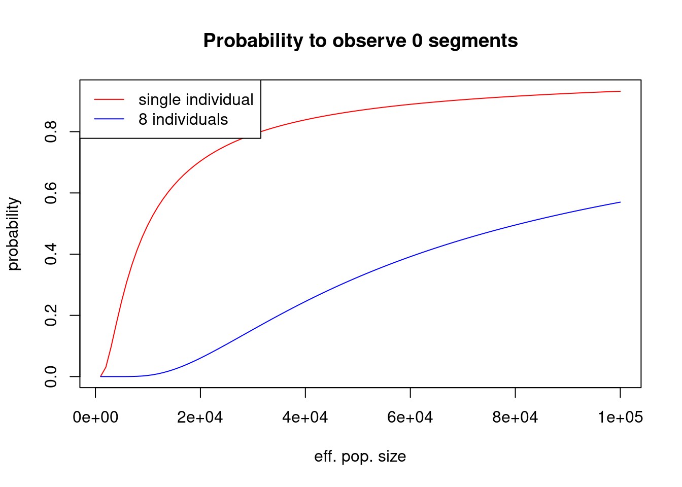
So we can see that for a single individual, the 0.05 threshold is passed for around \(N_e\approx 2000\) and for 8 individuals around \(N_e\approx 20000\). This makes sense: Absence of such segments in a single individual is less informative than in 8, requiring a larger effective population size to explain that absence in 8 compared to 1.
We can compute the precise threshold, too:
r <- uniroot(function(n) {n_roh_prob(0, 0.04, 0.08, n, 30) - 0.05},
             interval=c(500, 100000))
r$root
[1] 2317.825for a single individual, and
r <- uniroot(function(n) {n_roh_prob(0, 0.04, 0.08, n, 8*30) - 0.05},
             interval=c(500, 100000))
r$root
[1] 18747.53for 8 individuals
Exercise 3
Above, we have considered 0 segments, which allows only for a lower-bound estimate of population size. It gets more interesting when we actually do observe some segments. Again inspired by a real case, consider 8 individuals with a total of 6 segments between 2-4cM, so a shorter category. Plot the probability for this observation as a function of population sizes.
TipSolution
curve(n_roh_prob(6, 0.02, 0.04, x, 8*30), from=1000, to=100000,
      xlab = "eff. pop. size",
      ylab = "likelihood",
      main = "Likelihood to observe 6 segments")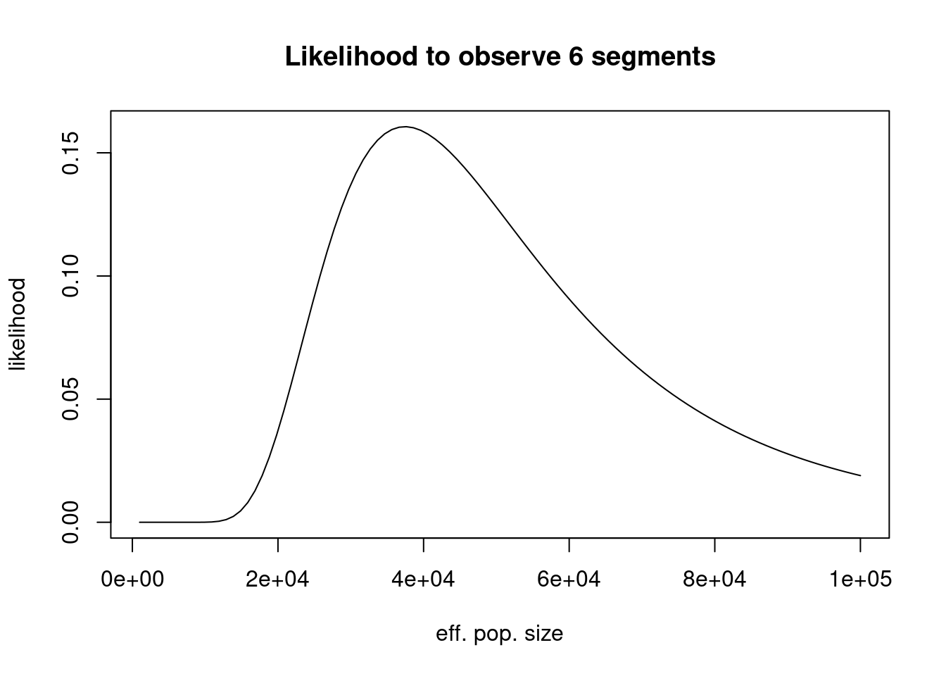
OK, so that looks like a nice bounded distribution. Note that this is not normalised to 1, as it is a likelihood (normalised over all possible observations, not over all parameters). We can normalise it to obtain a posterior distribution (assuming a flat prior):
norm <- integrate(function(n) n_roh_prob(6, 0.02, 0.04, n, 8*30), lower = 1000, upper = 100000)
curve(n_roh_prob(6, 0.02, 0.04, x, 8*30) / norm$value, from=1000, to=100000,
      xlab = "eff. pop. size",
      ylab = "probability density",
      main = "Posterior probability for Ne")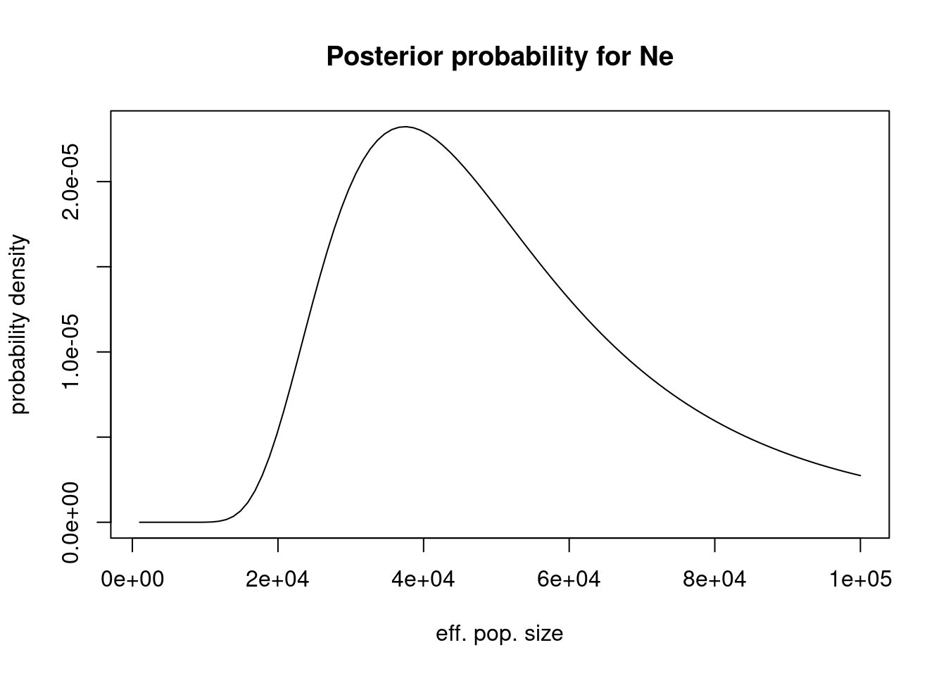
(note that integration should not start at 0, as the function is not properly defined for very low values of N).
We can also compute the cumulative distribution:
n_post_cumul <- function(n) {
    dens <- function(nn) n_roh_prob(6, 0.02, 0.04, nn, 8*30) / norm$value
    integrate(dens, lower = 1000, upper = n)$value
}
and use it to compute the 90% credibility interval:
uniroot(function(n) {n_post_cumul(n) - 0.05}, interval=c(1000, 100000))$root[1] 24176.97uniroot(function(n) {n_post_cumul(n) - 0.5}, interval=c(1000, 100000))$root[1] 46009.84uniroot(function(n) {n_post_cumul(n) - 0.95}, interval=c(1000, 100000))$root[1] 86153.5suggesting a median of \(N_e=36577\) with a 90% interval ranging from around 22000 to 48000, which is quite consistent with our lower bound computed from 4-8cM above.
Exercise 4
(Ringbauer et al. 2021) also computed the temporal distribution of time to common ancestors of ROH segments of a given length.
\(\frac{1}{2N}e^{-t/N}\left(e^{-2ta}(3 + 2Gt - 2ta) - e^{-2tb}(3 + 2Gt - 2tb)\right)\)
References
Carmi, Shai, Peter R Wilton, John Wakeley, and Itsik Pe’er. 2014. “A Renewal Theory Approach to IBD Sharing.” Theoretical Population Biology 97 (November): 35–48. https://doi.org/10.1016/j.tpb.2014.08.002.
Ringbauer, Harald, John Novembre, and Matthias Steinrücken. 2021. “Parental Relatedness Through Time Revealed by Runs of Homozygosity in Ancient DNA.” Nature Communications 12 (1): 5425. https://doi.org/10.1038/s41467-021-25289-w.